Condensate and feed water are heated in regenerative heaters by steam from uncontrolled turbine bleedings. Heating is carried out gradually due to distribution of steam extraction by pressure (the farther along the condensate (feed water) flow the heater is located, the higher the pressure of incoming steam). The heating steam condensate drainage is discharged either by gravity to a heater with lower pressure or by a condensate pump, depending on drain discharge scheme.
Introduction to the model structure
Consequences of level deviation in heater:
- A level decrease leads to steam slip, which can cause cavitation in the pump;
- A level increase leads to flooding of heat exchanger surfaces and deterioration of heat exchange, and increases the risk of water flooding into the turbine.
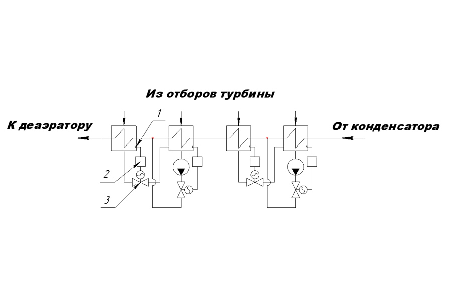
Level in all heaters is maintained by controllers 1 (Figure 1), which receive a pulse from level meters 2 and act on control valves 3.
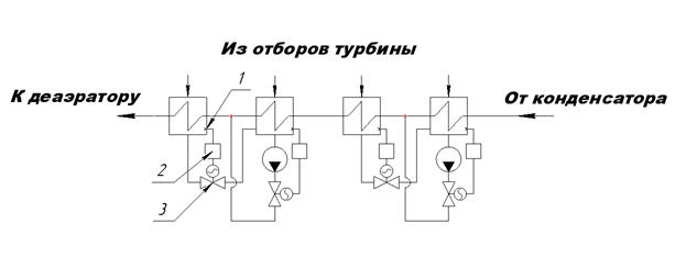
Figure 1. - Level control in regenerative heaters
|
К деаэратору |
To the deaerator |
|
Из отборов турбины |
From turbine bleedings |
|
От конденсатора |
From the condenser |
Control object
The first low-pressure heater (LPH-1) along the main condensate flow is selected as the control object.
Conducting simulation
Obtaining the acceleration curve
The acceleration curve is a change process in time of an output variable caused by a step input influence. The acceleration curve is used to identify the dynamic properties of the object.
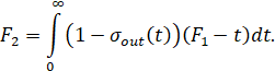
The model is preliminarily set to steady-state, then change of steam flow rate is simulated from 19.96 kg/s to 20.3 kg/s as a disturbing impact. Changing the flow rate leads to level change in the heater (see Figure 2).
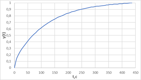
Figure 2. - Standardized acceleration curve (graph created in MS Excel based on available data).
Thus, the transient characteristic (acceleration curve) of the control object is obtained based on the IPA-1 model. This characteristic allows obtaining the transfer function of the object for further simulation of ACS (automatic control system) circuit in REPEAT software.
Obtaining the transfer function
An identification is the process of determining the mathematical model of a control object from experimental data.
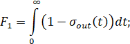
In order to identify the object parameters more accurately, the M.P. Simoyu method or "area method" is used, which allows to determine transfer function parameters from the acceleration curve of the object [1].
The method is based on the assumption that the studied object can be described by a dimensionless transfer function with constant coefficients 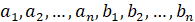 represented in the following form [1].
where:
 Laplace operator;
 rated output quantity;
 rated input quantity;
 denominator polynomial degree;
 numerator polynomial degree.
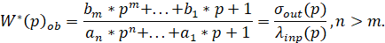
While using this method, the initial experimental acceleration curve is readjusted in the coordinates  , i.e., it is converted to a unit of output and input value in dimensionless form [1].
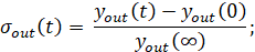
where:
 output value;
 input value.
This results in an initial characteristic in the range [0.1] (see Figure 2).
The identification function is to determine the unknown coefficients of the transfer function from the following system of equations
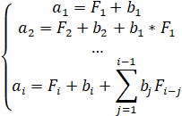
where:
 equation coefficients.
View of the desired transfer function
Then the system of equations

Coefficients are related to the transition function
  by the following ratios:
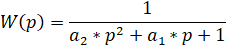
The object identification is completed by checking the accuracy of the experimental acceleration curve  and calculated from the found transfer function –
  [1]. Criterion for model adequacy
  :
:
where  – transient process time in the control object.
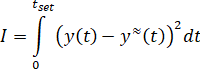
Implementation of the described algorithm using Python (see Figure 3).
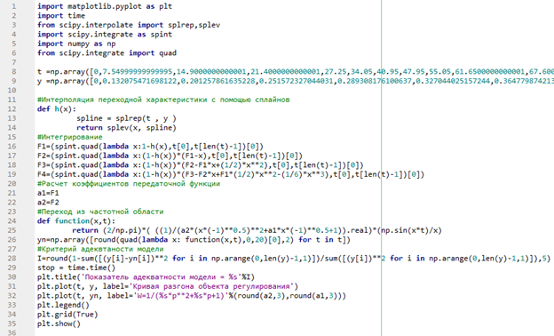
Figure 3. - Identification of acceleration curve by Simoyu area method
The obtained result is presented below (see Figure 4).
|
Показатель адекватности модели |
Model adequacy indicator |
|
Кривая разгона объекта регулирования |
Acceleration curve of the control object |
Figure 4. - Transient characteristic of obtained transfer function in Python IDE
Determination of PI-controller setting parameters
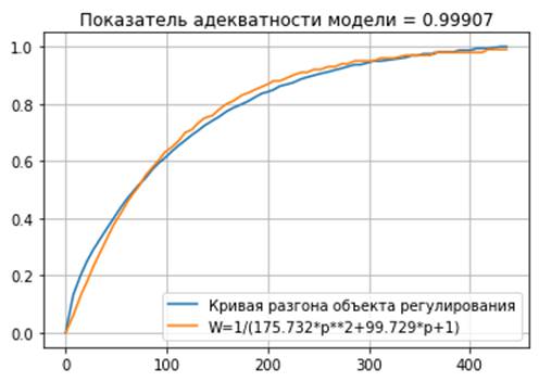
The controller is set up using the control and scipy libraries in Python. Optimization is carried out by finding the minimum of square of value deviation from the set point taking into account the control action.
The calculation algorithm using Python is given below (see Figure 5).
The obtained controller setting parameters:


Figure 5. - Optimization of PI controller parameters
Transient process
Simulate a closed-loop ACS with PI controller in REPEAT software – Figure 6.
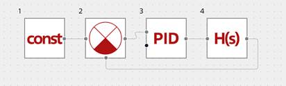
Figure 6. - Closed-loop ACS of level in LPH- 1
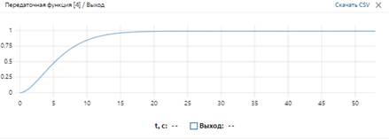
The obtained transient process is given below (see Figure 7).
|
Передаточная функция |
Transfer function |
|
Выход |
Output |
|
Скачать |
Download |
Figure 7. - Transient process (visualization in REPEAT software)
Transient process quality assessment
Assess the quality of the obtained transient process.
1) Dynamic error A1
According to the obtained diagram (Figure 6), there is no dynamic error.

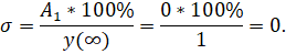
2) Over-regulation
3) Static error
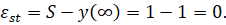
where  – setpoint signal value.
4) Degree of attenuation
No fluctuations.
5) Control time
The control time is  , the period after which the deviation of regulated quantity from the set value will not exceed a certain set value
  . It is assumed that

Then

6) Fluctuation period and number of fluctuations per control time
No fluctuations.
Simulation results
This article describes the process of obtaining a mathematical model of low-pressure heater as transfer function and developing an automatic control system of level maintenance in REPEAT software using Python libraries.
The transient process quality has been assessed. The transient process is stable and eliminates over-regulation, which will reduce the fluctuation of water level in the heater. Thus, based on the obtained results, it can be concluded that simulation results in REPEAT software are reliable.
References
- Identification and simulation of automation objects: lecture notes / A. V. Razzhivin, A. A. Serdyuk. - Kramatorsk: DGMA, 2011. - 124 pages.