Electric drive as a device is widely used in various applied and scientific fields. The most common ones are electrical machinery, radio electronics, automobile industry, automation engineering, and computer engineering. Multiloop circuits are used to simulate the operation of electric drives. The best and effective way is mathematical modeling of double-loop electric drive system, and REPEAT software being a model-oriented design and mathematical modeling environment successfully copes with these tasks of digital model creation. This paper describes the process of developing a DC double-loop electric drive system. Based on the given parameters, a suitable DC motor is selected. Using REPEAT software, a dynamic model of the electric drive is built based on the transfer characteristics of the electric motor, power supply (PS), current sensors (CT) and tachogenerator (TG) and a current and speed controller is synthesized. The simulation is examined using transient analysis and comparison with design values.

Input information for creating a simulation

Load moment of inertia Jl	215 kg ∙ m2
Static moment of load resistance Мl	145 N ∙ m
Angular velocity of load Ωl	44 deg/s
Required angular acceleration of load εl	9 deg/s2
Power supply transfer factor	24
Number of rectified voltage ripples per period m	3
Filter time constant	0.006 s
Input voltage of the current loop summing amplifier	8 V
Current sensor time constant	0.008 s
Input voltage of the speed loop summing amplifier	6 V
Tachogenerator time constant	0.007 s
Frequency of inverter supply voltage	400 Hz
Gearbox efficiency	0.85

Functional diagram of electric drive

The electric drive consists of a potentiometer, an amplifier, a DC motor (DC EM), a gearbox and a tachogenerator (see Figure 1).

The potentiometer is a control element. The control signals from the potentiometer output are transmitted to the input of the amplifier, with the armature winding of the DC EM with separate excitation being its load.

The EM turn the mechanism with angular speed proportional to the reference stimulus through the reducer.

Figure 1. Structural diagram of servo drive

The tachogenerator forms a rigid negative feedback (NFB) on angular velocity and ensures the signal generation at the amplifier input to deviate the load angular velocity from the design values.

This paper presents a closed-loop electric drive (ED) system based on the principle of REPEAT-based subordinate coordinate control. The system is multi-circuit, it consists of a speed loop and a current loop. Each loop of this system is configured separately.

Calculating of power and selecting of a DC motor

Based on the required parameters listed below, calculations are made for the selection of a DC EM and its dynamic model:

- required angular velocity of the load

- required angular acceleration of the load

- load inertia moment

- load static resistance torque ;

- gearbox efficiency .

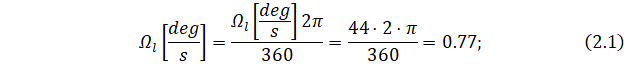
1. First, one should convert the angular velocity of the load rotation from “s” to “rad/s” and the angular acceleration of the load rotation from “deg/s²” to “rad/s²”:

The required power is calculated as follows:

2. EM with shaft rated power greater than the required power ( ˃ ) is selected.

Relative to the calculated parameters, electric motor MI-22F is selected. This motor is a DC reversible parallel-excitation actuator motor. It is designed for operation in automatic control circuits. Specifications are given in Table 1.

Table 1. Specifications of EM MI-22F

Motor type	Shaft power Prat, kW	Rotation frequency nrat, min-1	Supply voltage Urat, V	Armature current  Ia, А	Armature winding resistance Ra, Ohm	Rated torque Мrat, N ∙ m	Inertia moment Jmtr∙10–4 kg ∙ m2
MI-22	0,37	3000	110	4,4	0,546	1,2	40,8

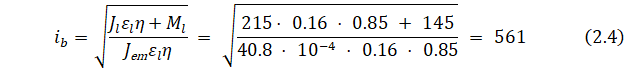
3. The best gear ratio   is calculated using the formula:

4. The selected EM is checked to ensure that it meets the speed requirements.

The following formula determines the rated angular velocity :

and the load angular velocity reduced to the EM shaft:

Since  the speed requirements are not met.

     A new gear ratio is calculated using the formula:

5. The required motor torque  is calculated:

6. The selected EM is checked for compliance with the torque (moment) requirements:

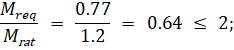
The torque requirements are met.

7. The parameters of the EM dynamic model are calculated.

   7.1. Counter EMF factor  is determined:

7.2. Torque factor  is determined:

7.3. The EM electromechanical time constant is determined:

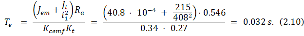
7.4. To determine the EM electromagnetic time constant the armature inductance  is calculated:

L_a = 0.0022 H is adopted to calculate the electromagnetic time constant  used in EM transfer function:

Electric motor parameters and factors are calculated:

Electromechanical factor:

Motor torque factor:

Electromagnetic factor:

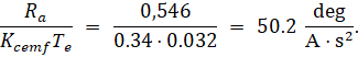
Taking into account the obtained numerical values of the dynamic model structural diagram, the EM DSSD appears as follows (see Figure 2):

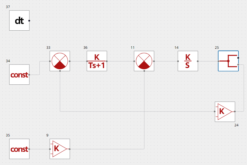
Figure 2. Structural diagram of dynamic model of electric motor with numerical values

Transient characteristics

Below the results of simulation with the following input parameters of EM Mi-22 are given (see Figure 3 and Figure 4).

- supply voltage U_rat = 110 V;

- rated torque M_rat = 1.2

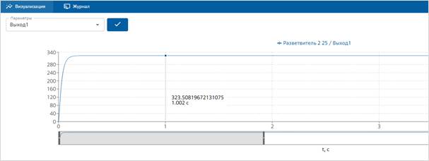
Figure 3. Reference stimulus transient characteristic of EM MI-22

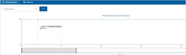
Figure 4. Disturbance transient characteristic of EM MI-22

Analysis of transients

Relative error is determine by the formula:

The data sheet rated value of angular rotation speed of EM MI-22 is and slightly differs from the simulation results (323.5 rad/s). It allows to conclude that the performed calculations are correct.

Current loop setting

The dynamic properties of PS are described highly accurately by a lag with a transfer function :

The dynamic properties of CT are also described by a lag

We can now present a dynamic simulation of the current loop based on REPEAT software (see Figure 5).

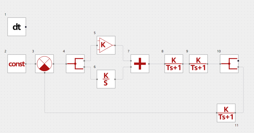
Figure 5. Structural diagram of the dynamic current loop simulation

Based on the structural diagram of the current loop simulation, the transfer function of the open current loop is found :

The current loop (CL) shall be adjusted to optimum modulo (OM). CL transfer function adjusted to OM:

where - is a total CL short time constant. To find it, a PS time constant is determined::

Then

To find the transfer function of the current controller (CC) it is necessary to equate the right parts of equations (3.3) and (3.4):

In terms of structure, the obtained equation is a transfer function of PI-controller:

Based on comparison of the last two formulas, we can obtain formulas to calculate a transfer factor Kcc and a time constant Тcc of СС:

To calculate the current transducer transfer ratio, use the formula:

To build a current loop according to (3.6), the current controller transfer function is calculated:

Transient characteristic

Preamble with indication (see Figure 6).

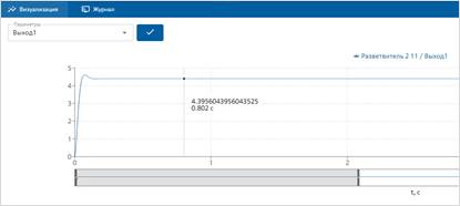
Figure 6. Transient characteristic of the current loop according to the reference stimulus (a CL reference stimulus is 8 V)

Transient analysis

Overshoot σ_cl and buildup time are determined..

The overshoot was calculated using the formula:

The expected overshoot when adjusting to OM

Based on Fig. 7 a maximum deviation of the armature current is determined:

and the steady state current value :

Overshoot is determined:

The overshoot corresponds to the correct setting.

The buildup time  is determined in the first point of intersection of the transient function graph and the armature steady state current value:

.

Based on the graph (Fig. 6) a buildup time is determined:

The buildup time can be calculated and should meet the requirement:

.

Deviation of measured and calculated value of :

The deviation is small and acceptable. One can conclude that the adjustment of the current loop to the optimum modulo was successful.

Adjustment of speed loop to symmetrical optimum

The speed loop (SL) consists of the following elements:

-       speed controller (SC) F1;

-       CL adjusted to OM;

-       motor electromechanical part;

-       tachogenerator (TG).

Before proceeding to the building of CL diagram, it is necessary to represent all loop elements in as links.

Dynamic properties of the TG (inertial link):

Adjustment of speed loop to symmetrical optimum (SO).

When adjusting SL to SO, due to short time constants T_ct and transfer function of the current loop

Transfer function of open SL :

where – is a SL total short time constant.

The transfer function of SL adjusted to SO is as follows:

To determine the SC structure it is necessary to equate the right parts of equations (4.3) and (4.4):

Let’s introduce designations to obtain the PI controller formula:

SC transfer ratio :

SC time constant:

Then the transfer function of the speed loop controller will be as follows:

The required TG transfer ratio is calculated using the formula:

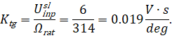
The transfer function of the speed controller is calculated using the formula (4.8):

A gearbox gear ratio is calculated:

Figure 7. Structural diagram of the dynamic speed loop simulation

Transient characteristics

Let’s build the output characteristics and analyze the results.

1. Building of SL transient characteristics based on reference stimulus. The value of SL reference stimulus is = 6 В.

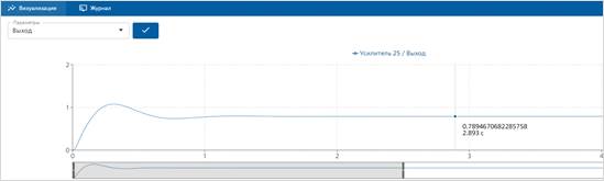
Figure 8. Reference stimulus transient characteristic of speed loop

2. Building of disturbance transient characteristic of SL (static moment of load resistance). Load M_l = 145 N/m.

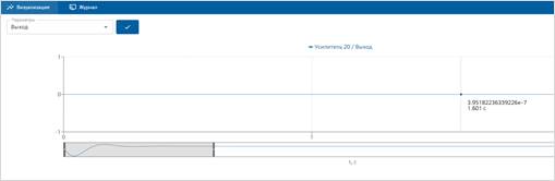
Figure 9. Disturbance transient characteristic of speed loop

The steady-state error component is reduced to zero.

Analysis of transients

Maximum deviation of the angular speed of motor shaft rotation and a steady-state value

Expected overshoot when adjusting to SO

Overshoot σ_sl:

Deviation from the expected value is and is adopted as acceptable.

and is adopted as acceptable. :

Calculated value :

Deviation of measured and calculated value :

Deviation of  is acceptable. The speed loop adjustment to the optimum modulo is successful.

Simulation results

This paper describes the development of the DC servo drive dynamic model and the synthesis of current and speed controller (double-loop system) using standard tuning methods such as modulo optimum and symmetric optimum. In the course of work, a DC electric motor MI-22F was selected.

REPEAT software was successfully used for creating a digital model. The simulation results and calculated values showed that the speed and current loops were set correctly with acceptable deviation values.